Tuesday, March 19, 2019

Perspectives on Teaching a Large Biology Class


This blog post is spurred on by some interesting conversations happening online about effective teaching and lecture prep strategies, so I though I would write something about my experiences over the last 8 years with teaching a large intro biology course, with the hope that some of this will be of use to others.

Our story begins in the Winter of 2011, my first semester teaching BI111 (Biological Diversity and Evolution), the 2nd half of the first-year biology courses (BI110, which runs in the Fall & focuses on Cells+Molecular Biology). BI111 has a broad course description (“Interactions of organisms with each other and with the environment in the ongoing process of evolution by natural selection are examined in the context of the interplay of form with function…”), which can be interpreted in any number of ways. I should also point out that I teach two sections of this course (in those days it was ~250-300 students in each, but now each section is ~450 students), and that while most students are in Science, the majority are NOT Biology majors (with the most common non-biology majors Kin, Health Science, Math, Chem, Psychology etc…), and as a result of all these different paths, not everyone in my class has taken grade 12 biology. So there is a wide range of prior experiences and reasons for taking this class.

As I mentioned, this class has a broad mandate, and the mistake I made in my first year was thinking that I should try and cover as much in the 2nd half of the intro bio textbook that I could. This sentiment is common in 1st year classes, with the idea being that you need to prepare students for any and all types of biology they may encounter in their second year. This is an obvious mistake, and quickly became apparent to me, as I tried to cram 2-3 chapters’ worth of topics into each week’s lectures (3 x 50min lectures/week x 12 weeks). Not only was I floundering at keeping up with the lecture prep, and because of the sheer amount of content, I couldn’t delve deep into any one topic during lectures. The course had already adopted the use of iClicker personal response devices, but my major use of them was for strictly ‘definitional’ questions (Which of the following best describes “term X”), and did not really test anyone’s knowledge.  The whole semester was nothing but stress and frustration, and the less said about it the better.

So at the end of this first semester I decided that I needed to fundamentally change up teaching strategy for this course. It is worth mentioning at this point, that the large number of changes I ended up adopting were not done all during the next year, but built up over time. This has only been achievable, as I have had the luxury of having a consistent yearly teaching assignment while at Laurier, allowing me to the time and opportunity to better develop each of the new elements. The first thing out the window was the “try and teach the totality of human knowledge” idea. Instead I decided to structure the class in such a way that I focused on fewer topics in a given week, and tried to make the topics covered in different weeks connect with each other. At the same time I made a conscious choice to move away from spending lectures defining terms, and instead use that time to apply the concepts associated with the definitions. This requires students to come into the classroom each week with at least a working knowledge of the key terms/ideas of the lecture, which meant that students should have read over the relevant textbook passages beforehand. This is an ongoing challenge for most profs, but I think I have solved it through the combined use of “Learning Objective” (LO) documents and “Entrance/Exit Quizzes”, which I will discuss below.

One of the biggest (logical & rational) concerns of an undergrad student is that they understand what they are expected to know in a given course. In an intro course, which covers many topics/chapters, this can be a big concern. So when I was redesigning the course, the first thing I did was go through my chosen textbook chapters (and other readings – more on that below), and create a Learning Objective Document, 
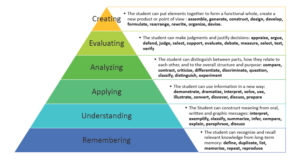
which is shared with the students at the start of the semester. This document has two sections (BASIC and ADVANCED), and are framed using Bloom’s Taxonomy words (you can see an example here: https://cpb-ap-se2.wpmucdn.com/global2.vic.edu.au/dist/d/8496/files/2015/09/Screen-Shot-2015-09-05-at-9.22.41-am-1jq2xw2.png, and another here: https://wp0.vanderbilt.edu/cft/guides-sub-pages/blooms-taxonomy
). The basic section focuses primarily on defining the terms I would expect everyone to be familiar with. The textbook does a great job at providing simple descriptions of concepts, and it would be redundant to spend lecture time repeating it. To ensure the students are familiar with these terms, on the weekend before the start of every week’s lectures I have a very simple online CMS-administered multiple-choice “Entrance Quiz” of ~8-10 questions based explicitly on the terms listed in the basic section of the Learning Objective document. This is a “low-stakes” quiz (not worth a large % of the course grade, but not very challenging)  that ends up having high participation (~90% on any given week), that also allows me to see (before the week’s lectures begin) if there are any terms that are tripping up students. Since lecture time is (largely) freed-up from going over simple definitions, this gives me more time to explore the week’s topic in more depth. This involves going into more detail than in the textbook, and apply their understanding of the definitions to new situations/contexts. These are more challenging tasks, and are mirrored in the “Advanced” section of that week’s lecture and focus on describing/explaining/discussing/predicting. At the end of each week I open up an online 8-10 multiple choice “Exit Quiz” that focuses on these advanced topics that runs over the weekend (and concurrently with the opening of the next week’s “Entrance Quiz). I have also recently started incorporating primarily literature reading into my course readings as the ability to read scientific papers is a skill that students will need in their future studies. For ~each week I have chosen a paper published in the journal Biology Letters, which have very short-form manuscripts (often 2-3 pages max) that are directly tied into the topic being covered in that week’s lectures (eg. 1, 2, 3), and can easily be swapped between years. An entrance quiz question may just focus on some simple term defined in the introduction or methods. During the week we would discuss the study in class, and an exit quiz question may be based on that discussion, or an extension of the experiment/study. Furthermore, I use (*and * tell my students that I use) the LO sheets when composing my mid-term and final exam questions, so that there are both short-term and long-term benefits of using them.

Now I want to emphasize that each of these elements takes time to construct, and can be a bit overwhelming if you were going to try and do it all at once. I think it would be perfectly fine if you developed the LOs in the 1st year, and then bring entrance and exit quizzes online in subsequent year(s).

So now that I’d freed up large chunks of lecture time, what to with it? Following the principle of ‘less is more’ I try to focus my time exploring on one or two key ideas in depth. Textbooks examples and definitions are pretty clear-cut, the result of lots of distilling and generalizing. I often try to show my students through case studies that things are not as simple. If we are talking about species concepts, I’ll go over the pros and cons of various concepts, and then present them with examples where (depending on the method used) they’ll end up with different conclusions. When discussing the general effects associated with plant hormones, I’ll ask them to hypothesize the likely changes in expression that have arisen between the ancestral and derived Brassica oleracea cultivars (broccoli, kale, kohlrabi etc..). I also try to use the lecture time to present physical examples of the lecture’s subjects. My classroom is equipped with a document camera, which is great because I can, for example, demonstrate to the students through dissections of flowers the various vegetative and non-vegetative whorls and structures, or by weighing slices of sweet potato that have been soaking in hypotonic or hypertonic solutions, how water moves across the plant cell membranes. I also use active learning exercises to illustrate how organisms/populations/communities change over time, with students playing different roles. Using iClickers and (lots of) playing cards, I can demonstrate the Hardy-Weinberg principle, and how violations of its assumptions change allele and/or phenotype frequencies; examine how selection leads to evolutionary change; how secondary growth proceeds in woodyplants; and the linkage of predator-prey population cycles. Again, this was not something I put in place overnight- my goal has been to develop/swap in 1-2 exercises per year. This gives me time to adequately develop the individual exercises (and reduces my stress level). This involves talking to my colleagues/grad students/undergrads about area where they see the greatest difficulties, then brainstorming about what would help. I am also very fortunate that Laurier has a great community of instructors and lots of institutional support.

OK. This ended up being longer than I expected, but I still think there is much more to discuss. Please feel free to comment below, and I will do by best to answer any questions you may have! I hope this has been of help!

TL

PS – If I can offer some other advice? Get yourself a digital audio recorder and a small wired “lapel/lapellier microphone, record all your lectures and put them immediately online your course’s website. Not only does help with accessibility issues, but it helps students out if they miss the occasional class, and/or if they can’t hear a key moment because of a local noise in the classroom.

PPS- If you are a BI111 student who has ended up here looking for more tips on how to do well in this class  - remember to look at your learning objective and (as always) read your syllabus!


Monday, January 22, 2018

Teaching about Adaptive Evolution: Battle of the Beaks


One of the important topics we cover in my BI111 (Biological Diversity & Evolution) class is the idea that Natural Selection leads to adaptive evolution. One way in which I teach this us this class (total enrolment ~800), is by a role-playing game I call the "Battle of the Beaks"

 The exercise is based specifically around the drought-related events described in of Boag & Grant (1984) Ecological Monographs 54:463-489. For this exercise I have purchased a number of pliers of various sizes from needle-nose through to pipe-wrenches (mostly from garage sales and/or dollar stores), as well as peanuts and walnuts* I start off by creating two teams of students with different sized-pliers. Typically each team is made up of 3 individuals (1 to be the "baby finch", who is to be "fed" by the "adult  finches").

 There are buckets of peanuts* at each of the classroom, and students have to run to the buckets, pick up peanuts, race back to the starting point, crush the shells to release the contents (one team member (the "baby") counts the number of nuts cracked). This is a race, to see how different beak teams perform in 2 minutes. This is meant to simulate a good year in the Galapagos. 

Next, to simulate what happens during a drought (when there is less food available, and what is left are primarily harder nuts), I break out the walnuts, and we re-do the competition between the teams. Now, the larger beaks have the advantage**. I then use this to talk about adaptive evolution, and specialization. Overall it is a fun and easy exercise that I highly recommend.


*This may be an issue for you if need to worry about allergies. This year was the first year I moved away from peanuts & walnuts and instead went to 2 types of beans (pinto & lima) + ping-pong balls (as the "large" seed).  Instead of crushing the seeds, the students could use their plier "beaks" to pick up the beads. The small beads will be easier to pick up, while the larger beads/marbles could only be picked up with the larger pliers. Alternatively you could marbles/beads of different sizes, or types of pasta. 

**Sometimes the results are not what you expect if you get a particularly competitive (or the opposite) team, so be prepared if the results are not what you might have been expecting!

Monday, January 8, 2018

Teaching Hardy-Weinberg & Population Genetics using playing cards


In-Class Population Genetics Exercise (note that this exercise will take more than one class to complete: at the end of 1st class, remind students to hold onto their cards).
To perform this exercise, you will need: i) a class of students; ii) sufficient playing cards so that each student can obtain 2 cards each (remove joker & instruction cards); iii) one distinct set of playing cards (that will be distributed among the sets); iv) everyone has a personal response system (PRS), i.e. an iClicker.

When cards are initially handed out to the students, DO NOT shuffle them, as we want initial population be in a state of non-H-W-equilibrium.

These cards represent (initially) a one gene, two-allele system. Hearts & Diamonds represent the red allele (r), while spades & clubs represent the black (B) allele. We initially treat B as dominant over r. (A real-life equivalent is the B & r alleles at the K-locus for coat colour in Cocker Spaniels). Each student represents a diploid individual, who is hermaphroditic (capable of mating with anyone else in the population).

Initial census of the class:
(For all calculations, I am assuming that the class is comprised of N=270 individuals –see accompanying excel file for other values).
Total starting population size of 270, most of which will be BB or rr.
Use clicker to 1st count phenotypes (Black or red) in population
Use clicker to then count genotypes.
Ask students to calculate p & q in starting population (should be p~0.5, q~0.5).

Simulation of Random Mating:
In this exercise, the point is to establish a population which is stable, and in which Hardy-Weinberg equilibrium becomes established

A new organism will replace each individual organism.
Ask students to turn to someone nearby, and to randomly exchange one of their two playing cards. This represents a reproductive event.

Using clicker, ask students what they think has happened to the frequencies of p & q (same as before, increase in p/decrease in q, increase in q/decrease in p, decrease in p/decrease in q, increase in p, increase in q).
Explain why p & q don’t change (no loss or gain of cards)

Ask students what they think will happen to phenotypes (same as before, increase in BLACK/decrease in RED, increase in RED/decrease in BLACK). Assuming that there will be more heterozygotes, we should see increase in Black phenotypes, and a decrease in Red phenotypes.
Poll students using iClicker to determine the distribution of RED & BLACK phenotypes in the population. Compare to initial distribution.

Ask students what they think will happen to genotypes (same as before, increase in BB & Br decrease in rr; decrease in BB increase in Br decrease in rr; decrease in BB, increase in Br decrease in rr, increase in BB decrease in Br increase in rr). Assuming that there will be more heterozygotes (due to random mating), we should see increase in Br phenotypes, and a decrease in BB & rr genotypes.

Poll students using iClicker to determine the distribution of BB, Br & rr phenotypes in the population.

At this point, discuss concept of H-W equilibrium: what is a model, why is it useful, what are its limitations (i.e. assumptions: sexually reproducing organism, reasonable large population, mating is random, no migration into or out of the population, no mutations, no selection

Use H-W formula to calculate predicted genotypes & phenotypes in the population. Compare these values to observations made in class.
Discuss why values may not match (mating was not fully random, finite population means no fractional individuals possible).

Get class to repeat random mating exercise as above. Use clicker to poll for phenotypes & genotypes. Discuss why or why not these frequencies have changed, and if they are getting closer to H-W equilibrium (hopefully they are).

Get class to repeat random mating exercise one additional time above. Use clicker to poll for phenotypes & genotypes. Discuss why or why not these frequencies have changed, and if they are getting closer to H-W equilibrium (hopefully they have). Use this data to indicate that as long as the assumptions are not violated, and that p and q remain constant, the genotype frequencies will hold constant at the Hardy-Weinberg equilibrium values, generation after generation.

Now, we want to see what happens if we start to violate the assumptions, starting with random mating.
Ask students to “mate” with others of the same phenotype (RED with RED; BLACK with BLACK). This is assortative mating.

Ask students what they think will happen to phenotypes/genotypes (same as before;
Increase in BLACK (more BB) decrease in RED; Increase in BLACK (more Br) decrease in RED, Decrease in BLACK (but more Br) increase in RED, Decrease in BLACK (but more BB) increase in RED.

Poll students using iClicker to determine the distribution of RED & BLACK phenotypes in the population. Were the results (hopefully Decrease in BLACK (but more BB) increase in RED) what people predicted?

Discuss how while mating in the whole population was non-random (assortative mating), that within the subset of BLACK phenotypes mating was random (because mating was based on phenotypes, not genotypes.
Assuming that there were (before the assortative mating) 135 Br individuals in the class & 67 BB individuals (H-W predicts 67.5), then for the 202 individuals (and 404 alleles in the population), there should be 269 B alleles (p=0.665) and 135r alleles (q=0.335). From these p & q values, we can predict how many BB, Br & rr individuals would be produced. BB: p2=0.44 (~89 individuals), Br: 2pq=0.44 (~89 individuals), rr: q2=0.11 (~23 individuals).

Ask students what would happen if we continued to have assortative mating? Changes in phenotypes/genotypes?

Now, get students to undergo dissortative mating (BLACK with RED, whenever possible).

Ask students what will happen to phenotypes/genotypes (same as before;
Increase in BLACK (more BB) decrease in RED; Increase in BLACK (more Br) decrease in RED, Decrease in BLACK (but more Br) increase in RED, Decrease in BLACK (but more BB) increase in RED. This should show how we get an increase in the amount of heterozygotes.

To show how random mating will restore population to H-W equilibrium, get students to undergo one round of random mating. Use iClicker to examine genotypes.

Next, we shall consider why a violation of the assumption of large population might affect our estimate of H-W equilibrium. Pick a row of ~10 students at random from the class, and get them to input (via iClicker, their genotypes). How close are their values to the p & q of the whole population and the predicted H-W values? Repeat with another row (this is to increase your odds of getting some atypical p & q values). This will show how small samples may not provide accurate representations.

Using a shuffled spare deck of cards, get 5-10 students to select 2 cards each at random from the deck. While p & q are=0.5, the observed frequencies of BB, Br & rr should (hopefully) not be in H-W equilibrium.

Next we shall consider effect of selection. Start by imagining that people don’t like RED Cocker Spaniels, and start only breeding BLACK dogs with BLACK dogs. This means that RED dogs don’t contribute to the next generation. Ask all students with 2 red cards to sit out the next mating round. Quickly survey the students on their genotypes before and after 2 rounds of mating (with any RED phenotypes) getting dropped from the population. Ask the students if they think that the r allele will be lost from the population selection against RED continues?

Demonstrate (using the rare (q=0.038) green-backed cards that have been mixed in with the regular black-backed cards q=0.962) how that even there is strong selection, that rate recessive deleterious genes will be retained in low frequencies (mostly as heterozygotic state). In a class of 270, there should be ~20 green cards in total, H-W predicts that there will be 0.38 individuals that are greenback/greenback (i.e.~0), 19.7 individuals that greenback/blackback are and 250 that are blackback/blackback. This means that >98% of green cards will be in heterozygous state (and hidden from selection).

Ask how the efficiency of selection would be affected if r or greenback alleles were dominant or co-dominant?

Next, let us consider selection acting on a quantitative trait (ask students to define quantitative vs. quantitative: perhaps asking them to write a list of 4 quantitative and 4 qualitative traits). Using the values on the face of the cards as allelic value (A=1, 2,3,4,5,6,7,8,9,10,J=11,Q=12, &K=13), get students to indicate phenotypic values (in clicker group into sets of 5: (2-6, 7-11, 12-16, 17-21, 22-26). Discuss the bell-shaped nature of the data: all value cards are in same proportions in the gene pool, but few outliers.

Perform directional selection (all those with values less than 7 must sit out) in two successive rounds of mating. Note how mean and distribution of population phenotypes changes.

Next, start stabilizing selection (all those with values less than 7 or more than 18 must sit out). Note how mean and distribution of population phenotypes changes.

If time permits, do several rounds of assortative mating and divergent selection: Selection for high values of BLACK, and low values of RED. Examine phenotypes over time.

Wednesday, June 14, 2017

My commencement address

 Today (June 14th) I received the Laurier Teaching Award for Sustained Excellence at the Spring 2017 convocation. As the recipient of this award I was asked to address the graduating class of Biology students (and their guests). I decided that it would be a good opportunity to talk about how success does not necessarily come easily. Specifically I wanted to focus on my initial difficulties with teaching http://www.ustream.tv/recorded/104772420
(starts ~38min mark)

------------------------  
It is a great honour to be the recipient of this award and I would like to thank all the individuals who nominated, supported and selected my nomination. As the recipient of this award, it is my privilege to be asked to give the commencement address for the class of 2017. Convocation is an excellent opportunity not only to celebrate your accomplishments, and to imagine the next steps of your journey, but also a chance reflect back on the challenges you have faced to get where you are today, and how you were able to overcome them. For me, receiving this award is –as I said- a great honour, but it also somewhat ironic, because it was not too long ago that I had serious doubts about my future as an educator.

When I began my position at Laurier it was with a great deal excitement and (and an equal amount of nervousness). Landing a tenure-track position was an amazing opportunity, and one that I (initially) thought I was well prepared for.  Throughout my graduate studies I had had the opportunity to work as a teaching assistant, and I had taken numerous elective courses and workshops on effective teaching practices. So I thought I would be able to at least hold my own when it came to teaching my first class. How wrong I was.

The first time I taught BI111 – Biological Diversity and Evolution – it felt like everything went wrong. I had taken over the course from a recently departed and much beloved instructor who I looked to as a model for how to run the course. But in that first class nothing clicked, nothing worked. As I stood in front of my sometimes confused, often bored, and occasionally frustrated, students I felt like a failure both professionally and personally. At the end of the semester my departmental chair came into my office – closed the door- and told me how worried she was for my future prospects at Laurier based on my teaching evaluations.

Now I don’t know if you – the class of 2017 – can empathize: Your first year at Laurier and getting much worse grades than you had been expecting based on you previous experiences – but I hope you can use your imagination.

Talking about failure is tough. Which is strange because we all encounter it. Far too frequently reality doesn’t match our expectations. For me it took some time to figure out how to identify why my teaching wasn’t working, and to start upon a better path. But I did not find my way along that path alone.

I am extremely fortunate to be surrounded by many excellent instructors both in my department and across the Laurier campuses who I have looked to for mentorship, for guidance and for conversation. I am here today because of Faculty, friends, and family members who shared with me their experiences and advice. I am also here because of some of the most important feedback I got was from my students on what they found effective, and what they found challenging. They inspired and encouraged me to take greater risks in my teaching. To imagine new approaches to learning about the amazing world in which we live, such as play-acting the process of secondary growth in eudicots, taking a busload of biostatistics students on a field trip to a literal field to collect their data, or learning the principles of Hardy-Weinberg equlibrium with thousands of playing cards (and the occasional pictures of cats). They helped me avoid getting discouraged if these experiments in teaching didn’t go as planned (which they sometimes did not).

And so here we are 6 years and roughly 4000 students later. I am on this stage because of the support of Laurier community and it is to them that I am eternally grateful. Class of 2017, today marks an important milestone in your lives.

For many of us in this room there will be challenges ahead, dark days in which you question your abilities and the path you have taken. Please remember you do not have to travel alone.  

Thank you

Monday, March 27, 2017

Thoughts on an predator-prey active learning exercise

Today was a very exciting day for me in my BI111 class, as I got to try out a role-playing game that I have been thinking / planning for a long while. At this point in the semester, my course (Biological Diversity & Evolution) has reached the topic of community ecology. One of the phenomenon I talk about this week is how predators and prey can become linked into cyclical patterns. A well-known example of this involves the  Candian Lynx, Lynx canadensis and its prey, the snowshoe hare, Lepus americanus. I've been wanting to try and let my students seem how this pattern, arises, so I devised an exercise that could be done in my two sections for BI111.
For context, this class has ~400 students per section, and I run i out of a lecture hall that holds 450 students (see pictures below)


Here is the set of rules I came up with, and shared with the students before today's lecture.

Now before you get too worried, I chose soft foam practice golf balls (I bought 4 sets from amazon) for use by the "lynx".

--------------------
OK. So, flash forward to the exercise in question. Overall. I felt it went well, but there are a few tweaks that I'm going to consider for next year's implementation.
1. Lynx - it was perhaps too easy for the lynx to survive and reproduce. In my 10:30 class, I followed the original plan, and it it didn't take long for the lynx population so rapidly rise. Things were a bit better in the second round, where I changed the rule to 4 hits =survival, 5=1 offspring and 6 hits=2 offspring. Lynx numbers still did increase pretty high, but it took a bit longer (I'll upload some scans of the data sheets later).
2. Hares. It became clear early on that the hares that survived needed bigger litters. Perhaps it was the orientation of the room, or the skill of the lynx at throwing, but predation success was greater than I anticipated. I tired out 3 offspring per litter. That seemed to work.
3.Time. I had expected that 5-6 rounds of predation + instructions preamble would take ~20 minutes (to give time for cycles to become apparent). It ended up taking about 30. Perhaps reducing the number of balls/lynx/round might speed things up.
4. Loundness. This was loud exercise. I knew it would, but - wow! Lots of excitement from the students (good), but hard to keep focus on the exercise. I'll need to think about what can be done.

That's it for now,  but I'll update this post when I get the student feedback on the exercise.
TL


Thursday, May 21, 2015

You are never too young (or to old) to be thinking about data visualization!

Over the last couple of weeks, I have been working with my son on his first science fair project. It has been lots of fun, working with him to develop a question, a prediction, and design a meaningful experiment. Collecting the data was also great - as you can (hopefully) see in the pictures below, we were investigating how rubber ball bounced at different temperatures. When it came time to "writing" up his results, we decided that the best approach would be to plot all his data (using stickers to represent the heights of the first bounce, of balls dropped from a height of 2m). While that may seem obvious, for many scientists, there is a great adversion to plotting raw data. It would be far more likely to see a "professional" version of this experiment present results using bar plots of mean values (and either SE, SD or 95%CI error bars). This is very unfortunate, as bar plots forsake a great deal of useful visual information about the distribution of the data. By coincidence, this was also (one of) the take-home message(s) of a recent paper:

Weissgerber, T. L., Milic, N. M., Winham, S. J., & Garovic, V. D. (2015). Beyond Bar and Line Graphs: Time for a New Data Presentation Paradigm. PLoS Biology: e1002128.


that we has chosen to read in this week's Long Lab journal club. Overall, I thought the authors did a commendable job, and it is evident from the paper's metadata that their message is reaching a large audience. While I am in favour of anything that turns the tide against bar plots, I do wish they would have given boxplots as much publicity as the univariate scatterplots that were heavily featured in the manuscript. I suspect that as the sample sizes in the literature they were surveying (physiology) tended to have small sample sizes  According to the authors "the minimum and maximum sample sizes for any group show in a figure ... were 4... and 10 respectively". These results are presented in panel C of supplemental figure S2*


I have nothing against univariate scatterplots. In fact, for small sample sizes (say <30 elements/group), directly plotting data reveals a great deal about the distribution of the data. However, after a certain point the usefulness of this approach starts to wain, as there will be more overlap in points. In such cases, a box-plot is a more desirable solution. Not only is as aesthetic, but is also clearly indicates meaningful visual information to the reader about the centrality, the skew and the distribution of the data. *I suspect that is why, when Weissgerber et al. presented their data of their hundreds of figures, they did so using a box-plot.

"let me tell you about the wonders of data visualization"

Tuesday, April 14, 2015

Statistically, it's mayhem*

Below is a letter to the editor I recently wrote in response to the potential flaws in the analysis that forms the basis of the Waterloo Region Record's recent article "Police call records reveal region's trouble hot spots" which can be read here ->http://goo.gl/DDQEg0

One of the first things that I emphasize to the students in my biostatistics class at Wilfrid Laurier University is that statistics are a powerful tool. Used carefully and properly, statistics can provide valuable insight into the factors that shape the world around us - but used or interpreted incorrectly, statistics can potentially lead to conclusions that are unjustified or altogether incorrect​. Your recent "analysis" of police call data seems to fall into the latter category due to problems with your data set, and in the conclusions drawn from them.

First, let's consider your data set. Of the ~903,000 calls in your initial data set almost half were excluded from the analysis for a variety of reasons. Whenever data is dropped, there is the strong possibility that what remains is a non-random (and thus biased) set of data. Furthermore, the remaining data points "do not measure crime" (as belatedly stated in the 30th inch of the story) -but instead capture a wide variety of incidents (including "enforcement of traffic laws" and "attend at collisions" that are not necessarily linked to the residents of that region). It should go without saying that if your data does not contain variables are relevant to the question, then the conclusions drawn from them will be suspect. 

Using this questionable data set, the conclusion "the poorer the zone, the more often people call police and the more time police spend there, responding to distress" is drawn, without any thought of potentially confounding effects. There are potentially dozens of other factors besides average household income that differ between the patrol zones that may be ultimately responsible for the observed patterns. For instance, a cursory search on Google Maps seems to indicate that the regions with the highest frequencies of calls to the police also have a greater density of Tim Hortons locations - but you would not (hopefully) conclude that their presence is responsible for "where trouble lives". 

Generations of statisticians have warned that "correlation does not imply causation", but that message seems to have been ignored in the construction of this article, to the detriment of your readership. 

Sincerely,

Tristan A.F. Long

*The title for this post is taken from one of the hyperbolic statements made in the article. I think that, ironically, this statement is an apt description of the statistics used in the analysis.